Vr Aerial Triangulation Tutorial, RPC Satellite Images
A tutorial for the Vr Aerial Triangulation Program (VrAt) (VrAirTrig)
See also: Vr Air Trig - Documentation
The Vr Aerial Triangulation program (VrAirTrig) allows the collection of strip and tie points on a large number of photos and performs a simultaneous bundle block adjustment. For RPC images, the bundle refines the coefficients provided with the images. Measured points can also be exported for adjustment in third party packages.
VrAirTrig provides a Layout window that enables the technician to arrange the project photos as if on a desktop. In the layout, users can view point readings, measure points, add control points, etc.
VrAirTrig's intuitive interface allows setting up, reading, and exporting aerial triangulation readings on up to 2000 photos.
Points may be measured in four modes mono-comparator, stereo, semi-automatic, and automatic.
First, create a 'New Project' in VrAirTring.
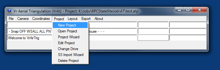
The software will prompt for a location and name, and then save an empty .atp file.
Immediately open the project in the 'Project Wizard'.
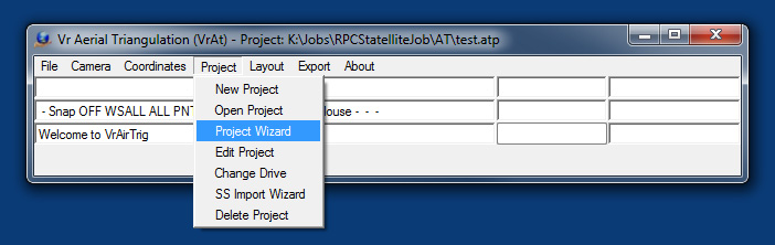
This will open the tabbed project wizard interface that steps through the setup process. Note that at any time Alt-S will save the project file. Clicking on the 'Save and Exit' tab will also save the project (and exit the project wizard). Clicking on the red 'X' at the top right will exit without saving.
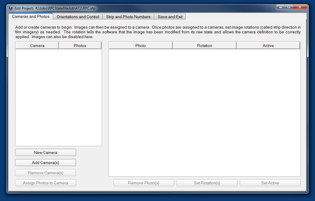
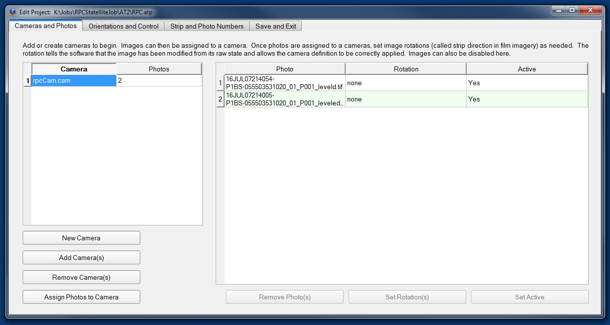
It is necessary to begin on the first tab of the project wizard by defining a camera file. All the photo based modules in VR require that images be associated with camera definitions. In order to support RPC within this convention a generic RPC camera is used. To create this generic camera click on the the 'New Camera' button. The edit camera dialog will open, and the camera type will default to 'Digital'. When the camera type is changed to RPC, all of the input fields will disappear (This is because all of the camera data is imbedded in the polynomial coefficients). Click 'OK' to save the RPC camera.

The new camera will be listed in the left table. Clicking on the number to the left of the camera name will select it; once a single camera is selected the 'Assign Photos to Camera' button becomes active. This button will open a file browse dialog that can be used to select the photos.
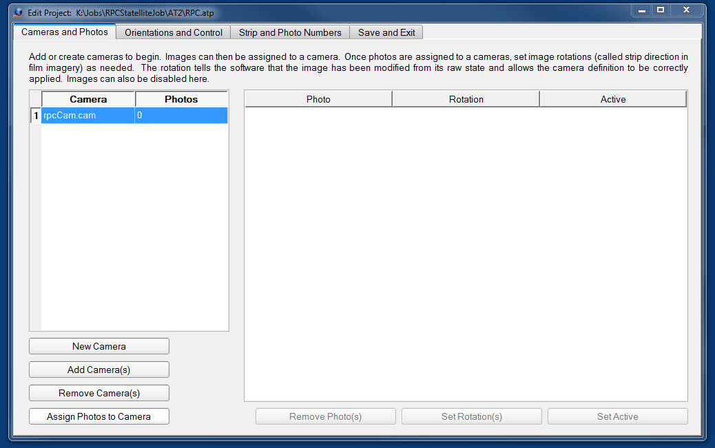
The photos will be listed in right table. This concludes the work in the first tab. Note that the images used in this example have been edited and saved with a '_leveled' postfix. The original images made very poor use of their dynamic range and were leveled in photoshop prior to processing. It is not yet known if this is typical.
Moving on to Project Wizard Tab 2, 'Orientations and Control'. The three buttons on the right of the tab correspond to the three operations that can be done here. The first 'Control File' is used to browse and find a control file. Any file of the format:
Name1 Lon1 Lat1 Height1
Name2 Lon2 Lat2 Height2
Name3 Lon3 Lat3 Height3...
Can be opened and used for the control file. The second button 'Import IOs' is not needed because IO's are automatic for any digital image including RPC satellite. The third button, 'Import EOs' is used to import the exterior orientations. The file browse dialog that will open lists all the available EO formats in a combo box at the bottom right.
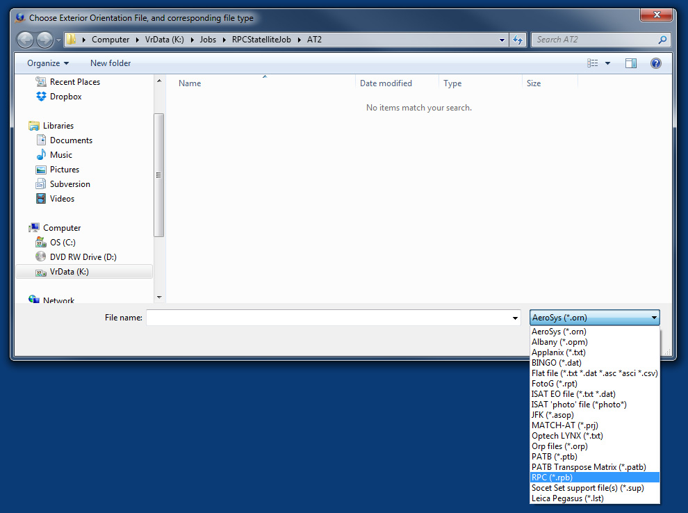
Currently there is only one format of RPC file supported, the .rpb provided with WorldView3 images. The reason for this, is that we only have example data from that sensor. More sensors will be added as clients request them.
Example WorldView3 rpb file:
satId = "WV03";
bandId = "P";
SpecId = "RPC00B";
BEGIN_GROUP = IMAGE
errBias = 1.11;
errRand = 0.27;
lineOffset = 6453;
sampOffset = 13833;
latOffset = 65.0682;
longOffset = -147.4682;
heightOffset = 486;
lineScale = 6454;
sampScale = 13833;
latScale = 0.0324;
longScale = 0.1495;
heightScale = 501;
lineNumCoef = (
+2.600687E-03,
+7.321254E-02,
-1.105985E+00,
+3.155668E-02,
+3.927141E-04,
-1.196724E-05,
+3.942317E-05,
-2.818333E-03,
-1.246034E-03,
-2.458765E-06,
-6.631219E-07,
+2.110715E-06,
+8.928089E-06,
+1.384127E-06,
-1.744533E-05,
-8.882365E-05,
-2.077458E-05,
+5.507292E-07,
+4.266188E-06,
+5.887024E-07);
lineDenCoef = (
+1.000000E+00,
+4.508323E-04,
+1.457076E-03,
-3.735878E-05,
+1.194044E-05,
+1.922784E-08,
+6.076005E-06,
+1.602818E-05,
-6.060599E-05,
+1.863469E-05,
+4.320563E-07,
+2.492354E-08,
-7.789835E-06,
+1.152282E-08,
-3.870810E-07,
+4.400122E-05,
+1.065839E-07,
+0.000000E+00,
-3.647255E-06,
+0.000000E+00);
sampNumCoef = (
-3.593168E-03,
+1.014127E+00,
+1.414506E-04,
-1.197804E-02,
-9.495031E-04,
+4.082122E-04,
-1.673931E-04,
+2.804113E-03,
+5.613618E-05,
+4.792464E-07,
+2.737975E-07,
-9.904634E-07,
-2.171797E-05,
-3.740261E-06,
+2.031331E-05,
+1.860997E-04,
+4.014185E-07,
+1.494090E-06,
-1.611103E-05,
+4.214402E-08);
sampDenCoef = (
+1.000000E+00,
+8.055703E-04,
+9.606289E-04,
-4.569766E-04,
-2.443157E-06,
-4.773518E-07,
-9.661562E-07,
+4.508436E-06,
+1.958310E-05,
-3.954105E-06,
+6.199317E-08,
-4.508929E-08,
-1.449302E-06,
+0.000000E+00,
+1.069904E-07,
+5.719918E-07,
+0.000000E+00,
+0.000000E+00,
-7.269755E-08,
+0.000000E+00);
END_GROUP = IMAGE
END;
Once a control file is selected and EOs are imported the tab should look similar to this.

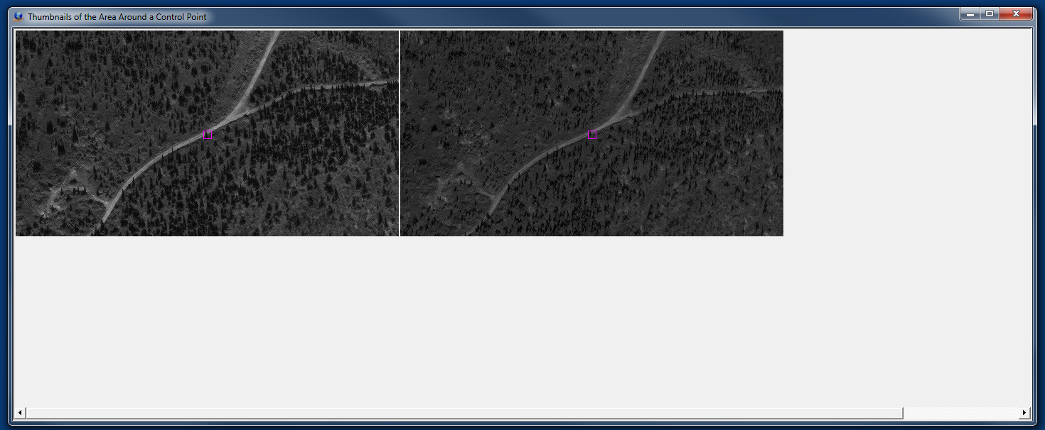
Notice the fifth column of the table titled 'Ctl Pts'. This column lists the number of control points that project into each image. Double clicking on one of the cells in this column allows user to view thumbnails of the control points in the images. If the image thumbnails look reasonable (as shown below) it demonstrates that the image EOs and control file are setup correctly.
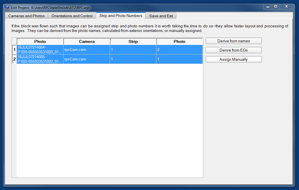
Moving on to Project Wizard Tab 3, 'Strip and Photo Numbers'. Strip and photo numbers are not really necessary. However, it takes only moment to assign them, and they may make project management easier. In this example, the two images were selected by dragging the curser down the row numbers to their left. The 'Assign Manually' button was then used to assign them to photo strip 1.
Project setup is complete. Alt-S to save and/or click on the tab "Save and Exit' to save and exit the project wizard.
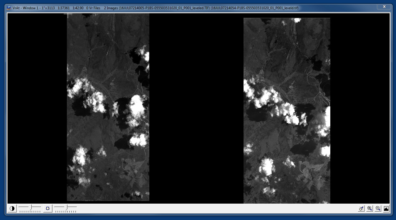
After project setup, the images can be opened in layout. If the images are not visible when you open the layout, click the 'Zoom All' button which is the extreme bottom right of the layout. To navigate in layout use the 'HOME' key to recenter the view and 'PAGE DOWN/UP' to zoom in and out.

Layout uses a 12 button menu navigation system. The buttons on the twelve key can be clicked with the mouse or activated using the F1-F12 keys on the keyboard. Also, the mouse left click is always linked to F1 and the mouse right click is linked to F2.
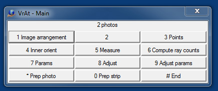
Upon clicking the button '1 Image arrangement' (or hitting F1) the menu will change to this.
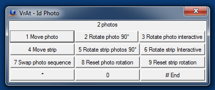
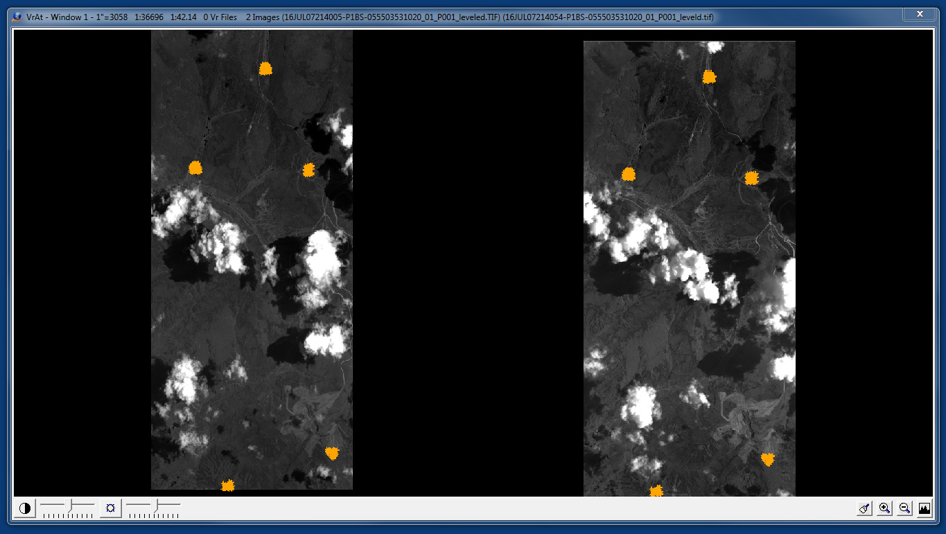
The nine active commands in this menu (F1-F9) are used by hovering the mouse over the images and pressing the F-Key for the command. They allow the images to arrange as desired. Note however that many layout functions will not work well if the images are overlapping. For very narrow images it may even be better to leave a little space between them. The '# End' key (or F12) will return to the Main menu. Here is an example of two arranged satellite images.
After the images are laid out as desired, navigate to the Add Points menu: Main->'3 Points'-> '1 Add Points Menu'.
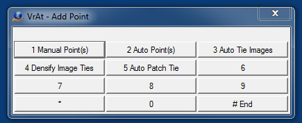
Use '5 Auto Patch Tie' (F5) to put in a few patches of points. To use this tool left-click on corresponding areas in the two images. Boxes will be drawn around the areas. Left click again to reposition a box. Right-click (or press F2 or click on the '2 Match patches' button) when satisfied to auto tie two areas. Below is a view of the layout with two patches ready to be matched.

Continue adding patches to define how the two images overlap as follows:
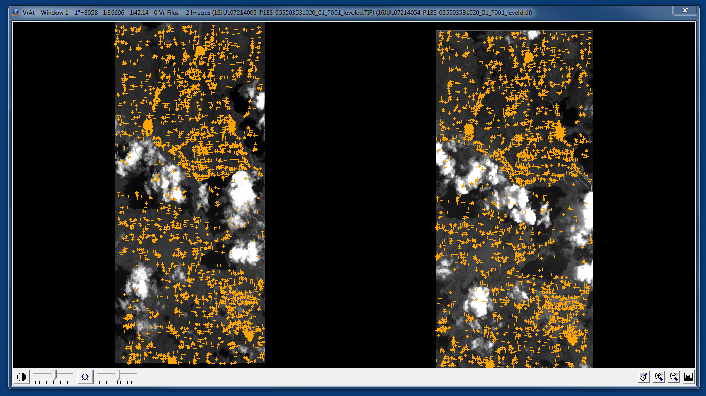
When the patches are finished the '4 Densify Image Ties' from the same 'Add Points' menu is used to fill in the rest. Left click on the button (or hit F4). Then left click on the two images, and finally right click to start the matcher. A parameter prompt will appear. For RPC images lots of data is recommended to prevent the solution from wandering away in areas with sparse data. In the example below 10,000 tie points are requested for this image pair. Note that '4 Densify Image Ties' can be run multiple times and additional patches or manual points can be added to fill in difficult areas.
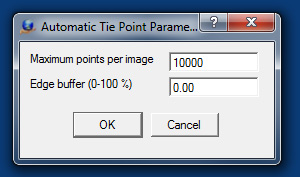
In this example '4 Densify Image Ties' was run twice because one corner of the images was sparse after a single run.
When satisfied with the point density use the Backup Atm command ('BacAtm') to save all the points. In case of any error these points can be restored using the ResAtm command. Then run a least squares match to refine and thin the data. Simply click through the bundle parameters menu (the bundle won't be run for RPC images). There are then two LS matching parameters
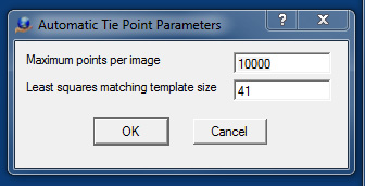
Again, for RPC images it is best to use a lot of points (10000 in this example). The template size can be varied. Large patches (60-200 pixels) will generate more matches and may be necessary in the trees. However, the matches will not be as precise. Small patches (10-40) will not be as numerous, but the precision will be better. For this example a patch size on the larger end of small (41) was used.
RPC images always start with exterior orientations so it is possible to drive to the control and measure it immediately after setting up the project. To open the drive control environment click on the button '6 Drive control' on the layout Points menu (Main->Points).
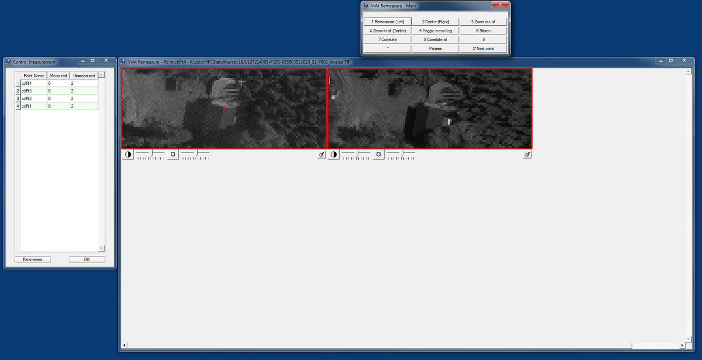
The two windows on the right of the drive control environment are identical to the point remeasure environment save for the '# Next Point' button. This button, as the name implies, loops to the next control point rather than exiting (as it would in remeasure). Otherwise everything is the same. Points can be measured in mono, stereo, or auto correlated. The red image boundaries indicate that the image points are only approximate. They will turn green as they are measured.
The table on the left provides overview and navigation. It lists all the control points, how many measurements there are of that point, and how many more measurements are possible. Clicking on column headers will resort the point order. Clicking on a point name will open that point for measurement. Clicking on the 'OK' button will exit the drive control environment.
To bundle in RPC mode use the command 'BunRpc'. The bundle interface has only two parameters:
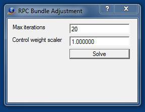
The 'Max iteration' can usually be left at default (20). The 'Control weight scalar' requires a little more explanation. A good way to think about is to remember that the error in the system does not go away when you bundle. It gets minimized, and the weights control how it minimized. In effect they allow the user to control how much error will show in the control matches as opposed to the tie points. The higher the 'Control weight scalar' the less error will be shown in the control point matches. However, error doesn't just go away. In this case it gets moved into the tie point matches, and high tie point errors can result in deformed models and Y-parallax in stereo viewing. So there is judgment required.
Here is an example of the output when running the bundle.
iter:0 maxCor:4.356907 RMSECtl:0.000000 RMSEtie:1.509726 VtPV:2.01e-005
Tie Res Percentile 0.1: 0.006578
Tie Res Percentile 0.2: 0.013701
Tie Res Percentile 0.3: 0.022311
Tie Res Percentile 0.4: 0.034669
Tie Res Percentile 0.5: 0.061657
Tie Res Percentile 0.6: 0.120365
Tie Res Percentile 0.7: 0.216336
Tie Res Percentile 0.8: 0.356033
Tie Res Percentile 0.9: 0.635720
Tie Res Percentile 1.0: 38.574399
iter:1 maxCor:0.743001 RMSECtl:0.000000 RMSEtie:1.514684 VtPV:1.56e-005
Tie Res Percentile 0.1: 0.004659
Tie Res Percentile 0.2: 0.009515
Tie Res Percentile 0.3: 0.015311
Tie Res Percentile 0.4: 0.023902
Tie Res Percentile 0.5: 0.038142
Tie Res Percentile 0.6: 0.071294
Tie Res Percentile 0.7: 0.138078
Tie Res Percentile 0.8: 0.223803
Tie Res Percentile 0.9: 0.426429
Tie Res Percentile 1.0: 39.331256
iter:2 maxCor:0.089789 RMSECtl:0.000000 RMSEtie:1.518507 VtPV:1.08e-005
Tie Res Percentile 0.1: 0.005192
Tie Res Percentile 0.2: 0.009886
Tie Res Percentile 0.3: 0.015313
Tie Res Percentile 0.4: 0.023956
Tie Res Percentile 0.5: 0.045626
Tie Res Percentile 0.6: 0.073249
Tie Res Percentile 0.7: 0.140855
Tie Res Percentile 0.8: 0.221256
Tie Res Percentile 0.9: 0.408954
Tie Res Percentile 1.0: 39.641716
iter:3 maxCor:0.011670 RMSECtl:0.000000 RMSEtie:1.520125 VtPV:1.02e-005
Tie Res Percentile 0.1: 0.004873
Tie Res Percentile 0.2: 0.009263
Tie Res Percentile 0.3: 0.014500
Tie Res Percentile 0.4: 0.023320
Tie Res Percentile 0.5: 0.033347
Tie Res Percentile 0.6: 0.067072
Tie Res Percentile 0.7: 0.129767
Tie Res Percentile 0.8: 0.209612
Tie Res Percentile 0.9: 0.398724
Tie Res Percentile 1.0: 39.849355
iter:4 maxCor:0.009927 RMSECtl:0.000000 RMSEtie:1.520495 VtPV:9.88e-006
Tie Res Percentile 0.1: 0.004656
Tie Res Percentile 0.2: 0.008936
Tie Res Percentile 0.3: 0.014276
Tie Res Percentile 0.4: 0.023103
Tie Res Percentile 0.5: 0.031537
Tie Res Percentile 0.6: 0.067422
Tie Res Percentile 0.7: 0.126841
Tie Res Percentile 0.8: 0.206983
Tie Res Percentile 0.9: 0.395114
Tie Res Percentile 1.0: 40.022998
iter:5 maxCor:0.008640 RMSECtl:0.000000 RMSEtie:1.520760 VtPV:9.75e-006
Tie Res Percentile 0.1: 0.004602
Tie Res Percentile 0.2: 0.008781
Tie Res Percentile 0.3: 0.014079
Tie Res Percentile 0.4: 0.022868
Tie Res Percentile 0.5: 0.030859
Tie Res Percentile 0.6: 0.065259
Tie Res Percentile 0.7: 0.123472
Tie Res Percentile 0.8: 0.206683
Tie Res Percentile 0.9: 0.394793
Tie Res Percentile 1.0: 40.192478
iter:6 maxCor:0.007140 RMSECtl:0.000000 RMSEtie:1.520989 VtPV:9.67e-006
Tie Res Percentile 0.1: 0.004453
Tie Res Percentile 0.2: 0.008742
Tie Res Percentile 0.3: 0.013954
Tie Res Percentile 0.4: 0.022851
Tie Res Percentile 0.5: 0.030597
Tie Res Percentile 0.6: 0.064318
Tie Res Percentile 0.7: 0.122338
Tie Res Percentile 0.8: 0.204505
Tie Res Percentile 0.9: 0.392674
Tie Res Percentile 1.0: 40.360051
'Tie Res' refers to the 2D error in the image point ties in pixels. Note first that the residuals are small. The 90th percentile (Tie Res Percentile 0.9) is less than half a pixel. Also, note that the median (Tie Res Percentile 0.5) starts at 0.06 and is reduced to 0.03. There are some large residuals (the max is 40.36 in this example). To eliminate the large residuals X out of the BunRPC gui. And go to layout Main->Points. On this menu the button '8 Show blunder points' opens a tool to view points by residual magnitude.
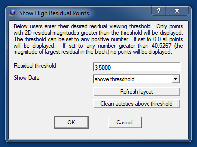
The 'Residual threshold' is the cut off for displaying points. 'Show data' allows the user to choose between showing data above the threshold (high residual data) or below the threshold (low residual data). The 'Refresh layout' button updates the layout view based on the threshold and above/below settings. 'Clean auto ties above threshold' deletes all auto ties with residuals above the threshold. Thus, viewing data above a threshold shows what data is to be deleted when cleaning. Showing data below the threshold shows the data that will remain after cleaning.
The following work flow is recommended.
1. Select a threshold that is high enough for the error to be obvious to the human eye (e.g. 5).
2. Refresh the layout to show points with residuals above the threshold.
3. Use the button '9 Remeasure point' to visually inspect some the points displayed. To do this click on the button and then double click a point. The remeasure window will open and display thumbnails of the point in all images. There is no need to actually fix the measurements. The whole intent is to determine if the points that the software is reporting as being in error actually are in error. To determine this, it is only necessary to sample a few points. If the points do not appear to be in error then there is likely insufficient data in the bundle or some other input issue. Assuming that the residuals reasonably reflect the apparent error continue to step 4.
4. Reset the 'Residual threshold' as desired. Use the display to check the point distribution, etc. When satisfied 'Clean autoties above threshold'. And 'OK' to exit. The general recommendation is to use a threshold somewhere at or above the 90th percentile. This gives a range of 0.4-40 pixels in this example.
5. Rerun the bundle (BunRPC) to see how the statistics have changed.
6. If desired repeat steps 1-5
After the bundle runs satisfactorily save the results ('Save' button). New RPCs will be saved to the image vim files (original files are not overwritten). The VrAt Project file (.atp) can now be opened in Vr Model Set and images setup for on-the-fly stereo viewing. Note, as the vim files are directly updated by BunRPC there is no need to import EOs in Vr Model Set.